Quantum Holistic Geology “Gas-QHG”, Discovered Natural Gas in Places Where it was said that it was Impossible.
Jose Vilca1*
1 Peru Aquaer Crys-Explo and San Agustín University, Perú.
*Corresponding Author:Jose Vilca, Peru Aquaer Crys-Explo and San Agustín University, Perú. Tel: 959342455; Fax: 959342455; E-mail: jcvilca45@gmail.com
Citation: Jose Vilca (2023) Quantum Holistic Geology “Gas-QHG”, Discovered Natural Gas in Places Where it was said that it was Impossible. SciEnvironm 6: 167.
Received: February 10, 2023; Accepted: February 20, 2023; Published: February 28, 2023.
Copyright: © 2023 Jose Vilca et al. This is an open-access article distributed under the terms of the Creative Commons Attribution License, which permits unrestricted use, distribution, and reproduction in any medium, provided the original author and source are credited.
Abstract
Year 2022, with OIL-QHG (José Vilca Post Doctorate, BGR, Germany, years 1983 to 1984) countries such as Russia, China, Argentina, now sell gas, because they have large reserves of this source of clean energy, thanks to technology that I developed, moreover, about 12 countries are joining in the search for the generation of gas in rocks of Paleozoic age, year 2022 (Why they did not do it before 2016, why recently), my gas exploratory technology was developed in the BGR, and Gas was discovered in Peru in 1984)with the support of a group of scientists from the BGR, I applied and developed a new analytical path at the BGR, Hannover, Germany, using the 10 samples from Peruvian rocks, which these pioneering geologists handed me over very in Secret, to be analyzed in the BRG, upon my return from Germany to PETROPERU in 1984.
Figure 1a: Shows the first Chromatogram of sample BGR CO11929 Paracas.
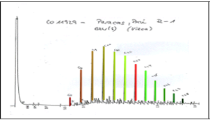
Peru: R-1 gtw (Vilca) and corroborated with the other nine samples of shales rocks and the tests with other laboratories like Girdel, France, and KFA, Julich, Germany, among others.
Figure 1b: They came directly to Camisea and not to another part of Peru, they had the adequate information that ensured the success of finding GAS in Camisea, Cusco, Peru in 1984.
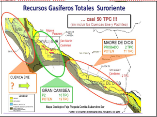
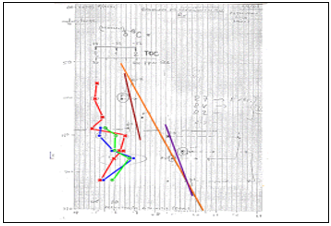
Figure 1c: It is the composite made by me, with the helped by of a scientist of the BGR: δ13C (Carbon 13 and Carbon 12 isotopes ratio) TOC (Total Organic Carbon Content) and SOL.
Conclusion
If it had not been for the courage to take the samples from Peru to Germany and the support of the German Scientists of the BGR, we would not now have large sources of energy like Russia and China and inputs for other industries. We would also not be exploring in very old Proterozoic rocks. then include, just in 2016 natural gas was discovered in Siberia Russia." Reconnaissance study of organic geochemistry and petrology of Paleozoic-Cenozoic potential hydrocarbon source rocks from the New Siberian Islands, Arctic Russia" then include, just in 2016 natural gas was discovered in Siberia Russia.
References
- Reconnaissance study of organic geochemistry and petrology of Paleozoic-Cenozoic potential hydrocarbon source rocks from the New Siberian Islands, Arctic Russia" then include, just in 2016 natural gas was discovered in Siberia Russia.
- A.P. Karpinsky Russian Geological Research Institute (VSEGEI), Sredny Av. 74, 199106, St. Petersburg, Russia.
- Federal Institute for Geosciences and Natural Resources (BGR), Stilleweg 2, 30655, Hannover, Germany.
- Institute of Geology, Leibniz University Hannover, Callinstraße, 30, 30167, Hannover, Germany.
- Total Explo EAC / PN, 2 Place Jean Millier, 92069, Paris La Defense, France.