Development of Automatic Sesame Grain Classification and Grading System Using Image Processing Techniques
Hiwot Desta Alemayehu1*
1Addis Ababa University College of Natural Sciences, Ethiopia.
*Corresponding Author: Hiwot Desta Alemayehu, Addis Ababa University College of Natural Sciences, Ethiopia, Tel: +251 11 123 9706; Fax: +251 11 123 9706; E-mail: hiwidesta7@gmail.com
Citation: Hiwot Desta Alemayehu(2019) Development of Automatic Sesame Grain Classification and Grading System Using Image Processing Techniques. Medcina Intern 3: 135.
Copyright: © 2019 Hiwot Desta Alemayehu, et al. This is an open-access article distributed under the terms of the Creative Commons Attribution License, which permits unrestricted use, distribution, and reproduction in any medium, provided the original author and source are credited.
Received: December 18, 2019; Accepted: December 29, 2019; Published: December 31, 2019.
Abstract
Sesame is one of the most important agricultural products traded internationally where its flow in the market needs to comply with the rules of quality inspection. Ethiopia is one of the largest producers and exporters of sesame in the world. The country produces three types of sesame grains: whitish Humera, whitish Wollega and reddish Wollega. To be competitive in the market, it is essential to assess the quality of sesame grains. Ethiopian Commodity Exchange (ECX) currently uses a manual grading system to assess the quality of the product. However, this technique is time consuming, expensive, inaccurate and labor intensive. Accordingly, it is essential to have an automated system which rectifies these problems. Thus, in this thesis, we present an automated system for classification and grading sesame based on the criteria set by the ECX.
The system takes pictures of sample sesame grains and processes the image to set the classes and grades. A segmentation technique is proposed to segment the foreground from the background, partitioning both sesame grains and foreign particles. The segmentation process also forms the ground work from which feature extractions are made. Color structure tensor is applied to come up with a better preprocessing, segmentation and feature extraction activities. Furthermore, watershed segmentation is applied to separate connected objects. The delta E standard color difference algorithm, which generates six color features, is used for classification of sesame grain samples. These six color features are used as inputs for classification and the system generates 3 outputs corresponding to classes (types) of Ethiopian sesame grains. Grading of sesame grain samples is performed using a rule based approach, where the classification output will be fed with 4 inputs and five or six outputs, corresponding to the morphological (size and shape) features and grades, respectively. On top of that, calibration is introduced to standardize the entire system.
Experiments were carried out to evaluate the performance of our proposed system design. The classifier achieved an overall accuracy of 88.2%. For grading of sesame grain samples, we got an accuracy of 93.3%, far better than the manual way of grading.
Keywords
Sesame Grading System, Digital Image Processing, Color Structure Tensor, Watershed Segmentation, Reconstructed Image, Delta E Color Difference, Calibration Process
Abbreviations
ANN- Artificial Neural Network; BP-Backpropagation; CIE-Commission International d'Eclairage; Delta E- Delta Empfindung; ECX-Ethiopian Commodity Exchange; HIS-Hue- Saturation- Intensity; L*a*b*- Luminance (intensity), redness-greenness and yellowness-blueness; RGB-Red-Green- Blue; SVM- Support Vector Machine
Introduction
Background: Sesame is one of the most ancient oil crops adapted to tropical and semi-tropical areas around the world. Ethiopia is known to be the origin as well as the center of diverse cultivated sesame commodity next to coffee in foreign exchange [1]. Major sesame production areas in Ethiopia are located in Humera, Metema and Wollo areas of the Amhara region, in Chanka and Wollega areas of the Oromia region and in Jawi areas of the Benshangul Gumuz region. Similarly, there is a considerable international market demand for Ethiopian sesame grain, and this is expected to continue increasing [2]. Ethiopia is endowed with different species of sesame grains. Among which the Humera sesame type is appreciated worldwide due to their white color, sweet taste and aroma. On the other hand, the high oil content of the Wollega sesame gives it a major competitive advantage for edible oil production [2].
The general broad types of Ethiopian sesame grains are classified into two:Whitish Humera Type: which has good demand in the world market and known for its top quality and quite large in size. It is also used as a reference for grading in the international market.
Wollega Type: which has high oil content.Sesame grain is the one of the exportable agriculture products found in Ethiopia. Thus, the quality of sesame grains is highly important for today’s market as some traders adulterate it with poor quality products. This malpractice has led to the production of low-grade quality sesame grains. Adulteration of grains may consist of mixing with stones, weed seeds, chaff, spoiled seeds and broken granules. This has been observed regularly in all sesame grains sold without proper inspection. This would badly affect the acceptance of Ethiopian sesame product on the international market [3].
Currently, the ECX offers an integrated warehouse system starting from accepting sesame grains to standardization. For example, in every warehouse, commodities are sampled, weighed and graded using grading and weighting equipment.
However, it is still a challenging task for ECX to keep similar quality level across the warehouses. Even if the ECX has grading laboratories and quality control specialists, a recent survey reveals that most of the customers are not satisfied with the quality, grading and sampling of commodities conducted in the warehouses. The reason behind this might be a lack of knowledge and lack of accurate measuring equipment [4, 5].
Nowadays, the process of classification and grading sesame grains have been done by experts using different techniques, such as visual inspection and weighting the sesame grains with scales. The ECX has implemented an approach which is a classical taxonomic approach to control the quality of sesame grain. This means, their classification and grading approach accuracy highly rely on human perception. However, this approach is time consuming, ineffective, expensive and labor intensive. Thus, considerable emphasis should be placed on keeping the accuracy of the grading technique in order to maintain the quality of sesame grains. Thus, a better way to control the quality and screen out the unwanted product effectively, an automated system of controlling is needed. Digital image processing is playing a big role in controlling and assessing the quality of agricultural products [6,7].
Motivation: The motivation behind this thesis is that though sesame is the second largest export commodity, Ethiopian sesame grain classification and grading is performed manually. As stated earlier, this technique has its own drawback, such as prone to error, labor intensive, aged and cost ineffective. Nowadays, this has become a big issue for ECX because it costs a lot of money and also causes to losing its reputation. In other words, it loses its market share on the international market. Thus, to be competitive in the market and proliferate its market share, it needs to improve the existing grading technique to compete with other countries.
This intrigue to come up with automatic way of grading the sesame grain based on their physical appearance. Statement of the problem: Ethiopia’s economy is highly dependent on agriculture, where 0.5% of its population are farmers. The ECX was established to modernize Ethiopian agricultural market and transform the economy through a dynamic, efficient and transparent marketing system.
Hence, maintaining the quality of a sesame grain is the main goal of ECX members and experts [5]. Dawit Alemu and W.Gerdien Meijer [8] pointed out that most of the exported sesame products have been facing several quality degradation problems.
Those problems might be due to lack of well-educated personnel, use of traditional grading technique and lack of advanced measuring equipment. On several occasions, different solutions were proposed by its members to overcome those problems, for example training the employees on regular based, upgrading the aged equipment and hire experts in those fields from other countries.
In line with this, the exactness of quality scrutiny via human assessment scheme is different from person to person according to the inspectors’ physical status such as working hassle, point of view and fidelity for traders [6]. In general, manual sorting, grading and classification which is based on traditional visual quality inspection performed by human operators are tedious, time-consuming, slow and inconsistent [6].
Few researchers have conducted an automated classification and grading system for different agricultural products such as coffee bean [9], wheat [10], maize [11], rice [12], fruits [13] and olive oil [14].
Literature shows that classification and grading technique proposed for an agricultural product will not be directly applied for others due to the difference in morphological, color and texture features.
To the best of our knowledge, there is no prior work attempting to develop a system for classification and grading of Ethiopian sesame grain. Thus, this research work aims at developing an automatic sesame grain classification and grading system taking the physical characteristics into account.
Objective
General Objective: The general objective of this research is to automate sesame grain classification and grading system using digital image processing techniques based on the criteria set by the ECX.
Specific Objective: The specific objectives of this thesis are:
Review literatures on previous works done on agricultural products and cereals., Collect sesame sample representing of the different features of sesame grain., Identify the best features of sesame grain that suits to a grading of sesame from various varieties of Ethiopian sesame production., Design algorithms for segmentation, feature extraction and grading., Design a classifier., Develop a prototype of the system., Test the effectiveness and appropriateness of the system.
Methods
In order to achieve the objectives different methods will be applied.
Literature Review: The literature review will be from different researches which are done on development of image analysis related to agricultural products. The other sources for detailed understanding of the sesame grain will be different articles on the issue, the Internet, organizational sesame grain specification document and books.
Sample Collection: It is necessary to have a sesame grain sample to carry out the thesis. The sesame grains will be collected from the ECX warehouse once they identified into their respective categories.
Prototype Development: To assess the performance of the system, its prototype will be developed. We will use Matlab for implementation. This will provide an insight on the applicability of the system. Moreover, to validate this prototype and the significance of the current work, testing and evaluation techniques will be used. Each experimental evaluations will measure using performance metrics and percentage accuracy measures.
Scope and Limitations: This research is limited to developing an automated grading system for the sesame grains before any post processing of the grain. On the basis of this, the physical property of sesame grain such as size, shape and color will be considered and does not include moisture and chemical content analysis.
Application of results: Some of the advantages of automated grading system are listed as follow:
It will minimize the processing time and labor cost. This will also improve quality based export of sesame grain., It gives a platform to conduct grading at one specific place, centralization. This in turn will enable ECX to have the same standard across all products and quality control will be easy., Minimize corruption that might rise due to manual grading so as the exporter or merchants may corrupt the grading experts., To reduce capabilities of decision-making that comes from human inspector physical condition such as fatigue and eyesight, mental state caused by biases and work pressure, and working conditions such as improper lighting, climate, etc., It will benefit researchers who need to take part in achieving the goal of developing efficient digital image processing techniques for different agricultural products.
Organization of the Thesis: The remaining of this thesis report is organized as follows. In Chapter 2, the literature review will be presented in brief. Chapter 3 discusses related works that had been carried out on automatic classification and grading of agricultural products. The design of automatic sesame grading system is presented in Chapter 4. The experiment, test results and discussion are presented in Chapter 5. In Chapter 6, conclusions, contribution of the thesis will be drawn and future works will be pointed out.
Literature Review
Introduction: These days, image processing is one of diagnostics techniques which grows dramatically. It forms core research area within engineering and computer science disciplines too. Currently, the use of digital image processing techniques has been exploded and applicable in many areas of interest such as medical visualization, law enforcement and inspection of the quality of agricultural products [6].
In this chapter, the literatures related to the concepts that are basis for this thesis are reviewed. First, we present an overview of Ethiopian sesame grains followed by grading techniques that are currently used by the ECX. Then, different techniques of image processing such as image acquisition, preprocessing, and different types of segmentation, feature extraction and classification are discussed in detail.
Ethiopian Sesame: Ethiopia is known to be the center as well as the origin of diverse types of sesame grains next to coffee [1]. This diversity in type and characteristic is the result of climate condition they planted. In recent years, Ethiopia’s sesame export share had grown from 1.5% in export quantity and 1.9% in revenue in 1997 EC to 8.9% and 8.3% in 2004 EC, respectively. In 2006, Ethiopia ranked 4th in export quantity and revenue following Sudan, India and China. This makes sesame one of the major source of foreign currency which in turn has significant impact on the growth and development of the country [1]. In general, there are so many types of sesame grain grown across the country, nevertheless only two of them are recognized on the international market. These are Humera and Wollega type sesame grain [1]. The diversity in characteristic can be illustrated as follows:
The Humera sesame grain has aroma and sweet test, the same size and quite large and whitish. As a result, the Humera type is distinctly called whitish Humera.
The Wollega sesame grain has high oil content and known to have two sub types identified based on their color as whitish and reddish Wollega.
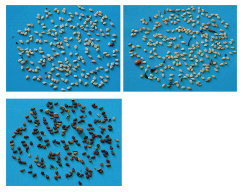
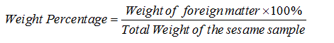
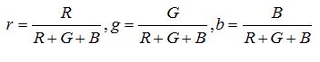
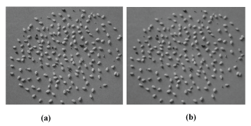
Sample sesame grain images from the three broad categories are shown in Figure 2.1. The top row from left to right shows samples of whitish Humera and whitish Wollega sesame grains whereas the bottom row shows sample of reddish Wollega sesame grains.
Figure 2.1: Samples of Sesame Grain Types
Practice of Sesame Grading in ECX: Currently, the sesame processing has two stages. This includes cleaning and hulling. The most common practice in Ethiopia is the export of cleaned raw sesame grain. Cleaning is the simple process of removing foreign material from the harvested sesame seed. Thus, it is a prerequisite for exporting raw sesame seed. However, the percentage to which the sesame grain has to be cleaned varies for different growing regions [14]. The first major component in the cleaning process is vibration screener which is used for selection of grains or similar products. At the same time, it separates dust and foreign materials. Secondly, the separation of stones is done by gravity separator which is especially designed to differentiate grains from granular material like little stones and other heavy impurities according to its specific weight [15].
Hulling is a process of removing the husk/skin from sesame grain after cleaning. There are two methods of hulling called dry and wet. Dry hulling is in which the sesame grains are dried and pounded to crack the husks. Wet hulling which requires soaking the sesame grains into water, pound, wash and dry it. Once the grains are hulled, they are passed through an electronic color sorting machine that rejects any discolored grains to ensure perfectly colored sesame grain [15].
Moreover, the grading system of sesame grain is fully dependent on both physical and internal composition of sesame grain. It should be free from any other odor, insects, mold and have to gain a moisture 10% of its weight [16]. ECX has developed its own classification of the varieties that are being traded on its grounds. Laboratories are set up in different locations that will classify and grades the sesame grains [16]. The technician will make a preliminary assessment of the product, in this case sesame in a restricted area on the premises but not in the warehouse to ensure: Uniformity of the capacity of the polypropylene bags (100kg) each., That there is no significant difference in the variety in all the polypropylene bags., There is no adulteration being committed., That there is no visible presence of insects and mold/fungus.
In light of this, the first step taken by the laboratory technicians are listed below: Physically evaluate the sample and evaluate the color, pest presence and mold presence., The second step is the screen size analysis which is done by the help of sieve like apparatus to check the size of each sesame grain. The analysis is carried out by adding 100g of sesame grain to the apparatus., Repeatedly shaking the gains on the equipment, the amount of sesame grains passed through the holes are weighted in-order to check the proportion of the sesame grain under the specified screen size.
The sample that is selected for further processing will undergo the grading process. The grading process will rely heavily on foreign matter [15].
The calculations being used in currently manual system in ECX is as follows:
 (1)
(1)
The continuous image function of the scene will process for representing digital images.
Let’s represent a continuous image function of two variables and suppose that we sample the continuous image into a 2D array, f (x, y), containing M rows and N columns, where (x, y), are discrete coordinates in which x is the horizontal position of the pixel and y is the vertical position. For notational clarity and convenience, we use integer values for these discrete coordinates: x = 0, 1, 2 … M - 1 and y = 0, 1, 2… N - 1. Thus, for example, the value of the digital image at the origin is f (0, 0), and the next coordinate value along the first row is f (0, 1). Here, the notation (0, 1) is used to signify the second sample along the first row. It does not mean that these are the values of the physical coordinates when the image was sampled. In general, the value of the image at any coordinates (x, y) is denoted by f (x, y), where x and y are integers. The section of the real plane spanned by the coordinates of an image is called the spatial domain, with x and y being referred to as spatial variables or spatial coordinates [17, 18].
Image displays allow to view results at a glance. Numerical arrays are used for processing and algorithm development. However, in equation form we write the representation of M×N in a more advantageous traditional matrix notation to denote a digital image and its elements [17]. Thus, Typically, there are distinct types of image types called gray-scale, binary, true color (red-green-blue). A gray-scale image is a 2D array of pixels (corresponding to the 2D array of cells), each pixel is a shade of gray, range from 0 (black) to 255 (white). This range means that each pixel can be represented by eight bits, or exactly one byte. Likewise, binary image is a logical array of 0s and 1s. Since there are only two possible values for each pixel, we only need one bit per pixel. Color images are images in which each pixel have a particular color, that color being described by the amount of red, green and blue in it using a 3D array [17, 19].
Dealing with this, the human eyes have adjustability for the brightness in which we can only identify dozens of gray-scales at any point of complex image, but can identify thousands of colors. In many cases, only utilize gray- scale information cannot extract the target from background we must by means of color information. Accordingly, the color image is a process of extracting from the image domain one or more connected regions satisfying uniformity (homogeneity) criterion which is based on features derived from spectral components.
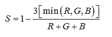
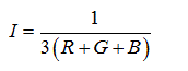
These components are defined in a chosen color space model [19]. The color is one of the most important features of information retrieval based on its content in the images. Color space or color model refers to a coordinate system where each color stands for a point. Many color spaces are in use today for pictures acquired by digital cameras. The most popular is Red, Green and Blue (RGB), Hue, Saturation and Value (or intensity) (HSI) and Luminance (intensity), redness-greenness and yellowness-blueness (L*a*b) model. In segmentation, reducing of dependence on changing in space lighting intensities is a desirable goal [19]. If variations of intensities are uniform across the spectrum then normalized RGB space is of value:
 (2)
(2)
Where, r is the red component, g is the green component and b is the blue component.
Next to this, we consider two possible alternatives coping with those difficulties, namely, HSI and L*a*b*. Both of them try to translate the human perception of color into figures. Besides, L*a*b* aspire to define a space where the Euclidean metric can be used straight away to estimate subtler color differences.
HSI color space model separates the color information of an image from its intensity information. Whereas, the perception of different intensity or saturation does not imply the recognition of different colors [19,20]. Next expressions compute those values from raw sensor RGB quantities:
![]() (3)
(3)
 (4)
(4)
 (5)
(5)
 (6)
(6)
Where, I model the intensity of a color, i.e., its position in the gray diagonal. Saturation S accounts for the distance to a pure white with the same intensity, that is, to the closest point in the gray diagonal. H is an angle representing just a single color without any nuance, i.e., naked from its intensity.
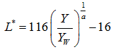
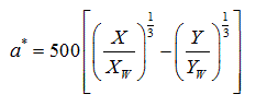
Moreover, the Commission International d'Eclairage (CIE) L*a*b has designed a uniform color space developed as a space to be used for the specification of color differences. It represents colors relative to a reference white point, which is a specific definition of what is considered white light, represented in terms of XYZ tristimulus space. These spaces are designed to have a more uniform correspondence between geometric distances and perceptual distances between colors that are seen under the same reference illuminant [20]. Measuring colors in relation to a white point allows for color measurement under a variety of illuminations. A primary benefit of using L*a*b* space is that the perceived difference between any two colors is proportional to the geometric distance in the color space between their color values. This is common in applications where closeness of color must be quantified [20].
Converting an image from RGB to L*a*b* results in the luminance or intensity of that image being represented on the axis named L that is perpendicular on a pile of ab planes. The values of the coordinates L*, a* and b* are real numbers when applying RGB to L*a*b* mathematical conversion. These values are mapped to integers from 0 to 255, making them somehow compatible with the 256 gray levels from each RGB color plane [20]. The mathematical conversion is defined from the tristimulus values normalized to the white defined by the following equations:
 (7)
(7)
 (8)
(8)
 (9)
(9)
Where, (X, Y, Z) are the tristimulus values of the pixel and (Xw, Yw, Zw) are those of the reference white. The approximation of these values from (R, G, B) by the linear transformation is given by:
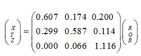 (10)
(10)
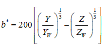
Our reference white is (Rw, Gw, and Bw) = (255; 255; 255). L* represents lightness, a* approximates redness-greenness, and b*, yellowness-blueness. These coordinates are used to construct a Cartesian color space where the Euclidean distance is given by:
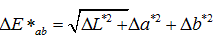 (11)
(11)
Where, E (Delta Empfindung) is a unit of measure that calculates and quantifies the difference between two colors and one a reference color.
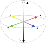
Figure 2.2 shows the three coordinates of CIE L*a*b* and their values represented on 3D. Where: The lightness of the color L* = 0 yields black and L* = 100 indicates diffuse white. Its position between red/magenta and green a*, negative values indicate green while positive values indicate magenta., Its position between yellow and blue b*, negative values indicate blue and positive values indicate yellow.
Figure 2.2: The L*a*b* Color Space as a 3D Cube
Digital Image Processing
An image may be defined as a two-dimensional function, where x and y are spatial (plane) coordinates, and the amplitude of ƒ at any pair of coordinates (x, y) is called the intensity or gray level of the image at that point. When x, y and the intensity values of ƒ are all finite or discrete quantities, we can call it as a digital image [21]. Image processing techniques can be used to enhance agricultural practices by improving accuracy and consistency of processes while reducing farmers manual monitoring. Often, it offers flexibility and effectively substitutes the farmers’ visual decision making. This is because machine vision systems do not only recognize size, shape, color, and texture of objects, but also provide numerical attributes of the object [21].
Grain quality attributes are very important for all users and especially the milling and baking industries. Computer vision has been used in grain quality inspection for many years [17, 22, 23].
Image processing and image analysis are the core of computer vision with numerous algorithms and methods available to achieve the required classification and grading. With this perspective, digital image processing focuses on two major tasks. These include improvement of pictorial information for human interpretation; and the other task is processing of image data for storage, transmission and representation for autonomous machine perception [24].
A computer-vision application using image processing techniques involves five basic steps such as image acquisition, preprocessing, segmentation, feature extraction and classification. This is illustrated in Figure 2.3
Figure 2.3: Digital Image Processing Paradigm
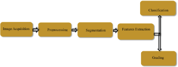
Image Acquisition
Before any video or image processing can commence, an image must be captured by a camera and converted into a manageable entity. This is the process known as image acquisition. Image acquisition is a process of retrieving a digital image from a physical source which is captured using sensors or cameras [18] since the quality of images will be affected through different factors. One of the challenges is the introduction of photometric invariants [18] such as shadow/shading and specularities. Consequently, the occurrence of inconvenient color illumination under different environment results in less quality image. Thus, to obtain the high accuracy quantitative and qualitative data processing, selection of image capturing sources and sensors have to be considered very carefully.
Preprocessing
Preprocessing is a sub-field of image processing and it consists of techniques to improve the appearance of an image, to highlight the important features and make more suitable for use in a particular application. The best result of this process will increase the classification accuracy of an object. Preprocessing techniques are needed on color, gray-level or binary images. Since processing color images is computationally high, character recognition system, most of the applications use gray or binary images. Such images may also contain non-uniform background and/or watermarks making it difficult to extract a feature of the image without performing some kind of preprocessing. Therefore, the desired result from preprocessing is a binary image [25,27].
However, an image may suffer some form of unwanted signal, noise. This unwanted signal changes the size and shape of the object of an image and blur the edge information. Noise may occur by physical condition of the system or may be due to environmental conditions. However, depending on the distribution of noise on the image, noise can be salt and pepper, Gaussian or speckle noise. Such degradation negatively influences the performance of many image processing techniques and a prepossessing step to remove the noise or to filter the image required [27]. As a result, noise removal and image enhancement processing is needed [27]. Median filter is the most common type of noise removal/filtering technique. Median filtering operation is used traditionally to remove impulse noise as it is the most commonly used in non-linear filter. It is easy to implement method of smoothing images. It works, first by sorting all the pixel values from the surrounding neighborhoods into numerical order and then replacing the pixel being considered with the middle pixel value. A 3*3, 5*5, or 7*7 kernel of the pixels is scanned over pixel matrix of the entire image [27].
Segmentation
Segmentation involves partitioning of an image into regions of corresponding to objects. All pixels in a region share a common property, for example simplest property that pixels can share is intensity [28]. Mathematically it can be expressed as:
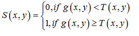 (12)
(12)
Where, S (x,y) is the value of the segmented image, g (x,y) is the gray level of the pixel (x,y) and T (x,y) is the threshold value at the coordinates (x,y).
The segmentation of an image I, which represents a set of pixels is partitioning into n disjoint sets R1,R2 …, Rn, called segments or regions such that their union of all regions equals I, I =R1 U R2 U …, U Rn . The most basic attributes for segmentation is intensity for a monochrome image and color components for a color image. Edge and texture of an image are also useful attributes for segmentation. The result of image segmentation is a set of segments that collectively cover the entire image [28, 29].
Typically, a good segmentation is the one in which: Pixels in the same category have similar gray-scale of multivariate values and form a connected region. Neighboring pixels which are in different categories have dissimilar values. Depending on the application areas, various image segmentation techniques have been proposed over the years. Among the commonly used segmentation techniques are thresholding, edge based segmentation, color structure tensor and watershed segmentation.
Thresholding
One of probably the most frequently used technique to segment an image is thresholding. Thresholding maps a gray-scale image to a binary image and the image fallen into two regions, naming by the pixel values 0 and 1 (255), respectively [28]. In this prospective, thresholding is used when the intensity distribution between the objects of foreground and background are very distinct. When the differences between foreground and background objects are very distinct, a single value of threshold can simply be used to differentiate both objects apart. Thus, in this type of thresholding, the value of threshold T depends solely on the property of the pixel and the gray level value of the image [30].
Edge-Based Segmentation
Segmentation can also be done by using edge detection techniques. Edges are detected to identify the discontinuities in the image. Edges on the region are traced by identifying the pixel value and compared with the neighboring pixels. Pixels which are not separated by an edge are allocated to the same category. When the objects show variations in their gray values, darker objects will become too small, brighter objects too large. The size variations result from the fact that the gray values at the edge of an object change only gradually from the background to the object value. No bias in the size occurs if we take the mean of the object and the background gray values as the threshold. However, this approach is only possible if all objects show the same gray value or if we apply different thresholds for each object. As a result, edge-based segmentation is based on the fact that the position of an edge is given by an extreme of the first-order derivative or a zero crossing in the second-order derivative [31, 32].
There are various edge detectors that are used to segment the image. The method used to segment image is called differential operator. Differential operator is a classic edge detection method, which is based on the gray change of image for each pixel in their areas. It is accomplished by the convolution. Sobel edge detector is one of the first-order differential operator [33]. Sobel edge detection operation extracts all of edges in an image, regardless of direction. It is implemented as the sum of two directional edge enhancement operations. The resulting image appears as a unidirectional outline of the objects in the original image.
Constant brightness regions become black, while changing brightness regions become highlighted. Derivative may be implemented in digital form in several ways. However, the sobel operators have the advantage of providing both a differencing and a smoothing effect. Because derivatives enhance noise, the smoothing effect is particularly attractive feature of the sobel operators [33]. Figure 2.4
Figure 2.4: Sobel Kernel
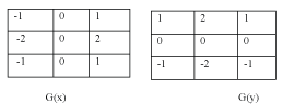
The operator consists of a pair of 3×3 convolution kernels as shown in Figure 2.4. One kernel is simply the other rotated by 90°. The kernels can be applied separately to the input image, to produce separate measurements of the gradient component in each orientation (Gx and Gy).
The gradient magnitude is given by:
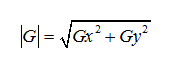 (13)
(13)
Typically, an approximate magnitude is computed using:
![]() (14)
(14)
Which is much faster to compute.
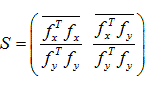
Color Structure Tensor Based Segmentation
Tensors are simply mathematical objects that can be used to describe physical properties, just like scalars and vectors. The structure tensor is often used in image processing and computer vision where it is used as a matrix representation of partial derivative information of an image. These partial derivatives of images represent the gradient or edge information of the image [34].
Simply summing differential structure of various color channels may result in cancellation even when evident structure exists in the image. Rather than adding the direction information of the channels, it is more appropriate to sum the orientation information. Such a method is provided by tensor mathematics for which vectors in opposite directions reinforce one another. Tensors describe the local orientation rather than the direction. The tensor of a vector and its 180º rotated counterpart vector are equal. For that reason, the structure tensor is a basis for color feature detection [34].
Given an image f, the structure tensor is given by:
 (15)
(15)
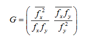
Where, the subscripts indicate spatial derivatives and the bar _: indicates the convolution with a Gaussian filter. Hence, there are two scales involved in the computation of the structure tensor. Firstly, the scale at which the derivatives are computed and secondly the tensor-scale which is the scale at which the spatial derivatives are averaged. The structure tensor describes the local differential structure of images, and is suited to find features such as edges and corners. Besides, tensors can be added for different channels such as multichannel image f = (f1, f2…,fn) T.
Hence, the structure tensor in Equation (15) will be rewritten as:
 (16)
(16)
Where, superscript T indicates the transpose operation for color images f = (R; G; B) T. This results in the color structure tensor:
 (17)
(17)
The color structure tensor describes the 2D first order differential structure at a certain point in the image.
Eigenvalue analysis of the tensor leads to two eigenvalues which are defined by:
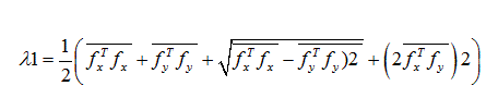 (18)
(18)
 (19)
(19)
Where, λ1 is the first eigenvalue and λ2 represents the second eigenvalue.
The direction of λ1 indicates the prominent local orientation which is equal to the orientation in the image with maximum color change.
 (20)
(20)
The two eigenvalues λ1, and λ2 are values in the local orientation which are the most and least prominent orientation respectively. λ1 - λ2 describes the derivative energy in the prominent orientation is corrected for by energy contributed by noise, λ2. An ideal linear symmetry is present in the image, when value of the two eigenvalues, λ2 = 0 and λ1 > 0. Besides, the λ’s can be combined to give local descriptors. The sum of λ1 and λ2 describes the total local derivative energy [34, 35]. ????20 is the vector in the direction of the largest eigenvalue. The vector ????20 can be computed directly from the complex tensor as:
![]() (21)
(21)
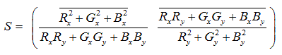
Where, S is the complex structure tensor defined in Equation 16. However, in color tensor the spatial derivative in the direction of x and y should be applied for all color channels as follow:
???????????? = (????????+????????+ ????????)
???????????? = (????????+????????+ ????????)
Where, R, G, B define the corresponding red, green, and blue channels respectively. Therefore, we can drive the vector ????20 for three channels by applying Equation 17 to equation 21 as follows:
![]() (22)
(22)
Where, ????????????: represents the convolution of the sum of the square of the spatial derivative in the direction of x.
????????????: represents the convolution of the sum of the square of the spatial derivative in the direction of y.
????????????: represents the convolution of the sum of the product of the partial derivative in the direction of both x and y.
Furthermore, the basic approach to color images the gradient is computed from the derivatives of the separate channels. The derivatives of a single edge can point in opposing directions for the separate channels. A simple summation of the derivatives ignores the correlation between the channels. Thus, this also happens by converting the color image to luminance values. In the case of luminance of adjacent color regions, it will lead to cancellation of the edge. As a solution to the opposing vector problem, leads to propose the color tensor for color gradient computation. The changes in the reflection manifest themselves as edges in the image. There are three causes for an edge in an image. These are an object change, a shadow-shading edge and a specular change. This information is used to construct a set of photometric variants and quasi invariants [34, 35].
Photometric invariance is important for many computer vision applications to obtain robustness against shadows, shading and illumination conditions. A good reason for using color images is the photometric information which can be exploited. It provides invariants for different photometric variations. Well known results are photometric invariant color spaces such as normalized RGB or HSI. Opposing derivative vectors are common for invariant color spaces. Actually, for normalized RGB the summed derivative is per definition zero. Hence, the structure tensor is indispensable for computing the differential structure of photometric invariant representations of images [35].
The derivative of an image is projected on three directions called variants. Therefore, the projection of the derivative on the shadow-shading direction results in the shadow-shading variant. By removing the variance from the derivative of the image, we construct a complementary set of derivatives called quasi-invariants. These quasi-invariants are not invariant with respect to a photometric variable. However, they share the nice property with normal invariants that they are insensitive for certain edges, e.g., shadow or specular edges [35]. The commonly applied feature detector, which is based on the structure tensor in computer vision, is the Harris corner detector. The color Harris operator H on an image f can be computed using Equation 23.
 (23)
(23)
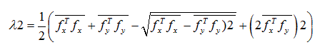
Figure 2.5 shows shadow-shading invariant images (b) and quasi-invariant resultant images (c) for a given color image (a).
Watershed Segmentation
Watershed algorithm is a region based segmentation technique. Its algorithm is more representative and iterative adaptive threshold algorithm in the application of mathematical morphology theory [28]. Obviously, segmentation of images involves sometimes not only the discrimination between objects and the background, but also separation between different regions. One method for such separation is known as watershed segmentation. Several works used watershed segmentation to isolate overlapped objects. The idea of watershed algorithm is from geography consider an image f as a topographic surface and define the catchment basins and the watershed lines in terms of a flooding process. Imagine that each cavity of the surface is pierced and the surface is plunged into a lake with a constant vertical speed. The water entering through the holes floods the surface. The moment that the floods filling two distinct catchment basins start to merge, a dam is erected in order to prevent mixing of the floods. The union of all dams defines the watershed lines of the image f [28]. In one dimension, the location of the watershed is straightforward, and it corresponds to the regional maxima of the function. In two dimensions, one can say in an informal way that the watershed is the set of crest lines of the image, emanating from the saddle points. The method stick this initial contour to the maximum contained watershed contour. For label image G = [R, E], we assume each edge eij ? E is a directing curve with the direction the same as clockwise direction of region Ri’s contour [32].
In light of this, after the necessary segmentation techniques are applied on a sample image, morphological operations are used to measure and extract the image correspond shape, achieve the image analysis and identification purposes using a certain form of structuring elements. It can be used to simplify the image data, maintain the basic shape of the image features and at the same time remove the image has nothing to do with the part of the research purposes. A common practice is to have odd dimensions of the structuring matrix and the origin is defined as the center of the matrix. Structuring elements play in morphological image processing the same role as convolution kernels in linear image filtering. When a structuring element is placed in a binary image, each of its pixels is associated with the corresponding pixel of the neighborhood under the structuring element [33]. The structuring element is said to fit the image if, for each of its pixels set to 1, the corresponding image pixel is also 1. Similarly, a structuring element is said to hit, or intersect, an image if, at least for one of its pixels set to 1 the corresponding image pixel is also 1. Zero-valued pixels of the structuring element are ignored, i.e., indicate points where the corresponding image value is irrelevant. The four basic morphological operations, namely erosion, dilation, opening and closing are used for detecting, modifying, manipulating the features present in the image based on their shapes. Based on these basic operations can also be combined into a variety of morphological methods to calculation [32]. The key of morphological operation, is how to combine morphological operator and use the morphological structure of various basic operations, how to select the structural elements to better solve the edge detection accuracy and the coordination of anti-noise performance [33].
Feature Extraction
After segmentation is done, feature extraction is the next major step performed in preprocessing of image. Feature extraction concerns finding morphological features such as shape and size and color features in digital images. The most important ones, are minor axis length, major axis length, eccentricity, area and perimeter [36].
Major Axis Length (Major): It is the distance between the end points of the longest line that could be drawn through the sesame grain. The major axis end points are found by computing the pixel distance between every combination of border pixels in the sesame grain boundary and finding the pair with the maximum length [36].
Minor Axis Length (Minor): It is the distance between the end points of the longest line that could be drawn through the sesame grain while maintaining perpendicularity with the major axis [36].
Area: is defined as the number of pixels contained within its boundary. Area is computed by counting the total number of pixels belonging to the object in the binary image. If we do pixel by pixel walk around the edge of the object, we are computing its perimeter. The perimeter of the image is the length of its boundary [36].
Eccentricity: is a parameter associated with every conic section. The eccentricity is the ratio of the distance between the focal points of the ellipse and its major axis length [36].
Classification
Image classification is perhaps the most important part of digital image analysis. The classification of agricultural products is determined by classifying them into different classes according to their quality. All classification algorithms are based on the assumption that the image in question depicts one or more features and that each of these features belongs to one of several distinct and exclusive classes [37]. The two main classification methods are supervised classification and unsupervised classification. In supervised classification, we identify examples of the information classes of interest in the image. These are called as training sets [38]. Unsupervised classification is a method which examines a large number of unknown pixels and divides into a number of class based on natural groupings present in the image values. Unlike supervised classification, unsupervised classification does not require analyst-specified training data. Rather, this family of classifiers involves algorithms that examine the unknown pixels in an image and aggregate them into a number of classes based on the natural groupings or clusters present in the image values [38]. One common form of clustering, called the K-means. This approach accepts from the analyst the number of clusters to be located in the data. The algorithm then arbitrarily locates, that number of cluster centers in the multidimensional measurement space. Each pixel in the image is then assigned to the cluster whose arbitrary mean vector is closest. After all pixels have been classified in this manner, revised mean vectors for each of the clusters are computed. The revised means are then used as the basis of reclassification of the image data.
The procedure continues until there is no significant change in the location of class mean vectors between successive iterations of the algorithm. Once this point is reached, the analyst determines the land cover identity of each spectral class [37]. Depending on the application areas, various supervised classifiers have been proposed over the years. Among the commonly used supervised classifiers are Navie Bayesian, Support Vector machine (SVM), Artificial Neural Network (ANN) and C4.5.
Naive Bayesian classifier
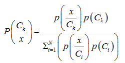
Naïve Bayesian is a classifier which is based on probability distribution. It classifies an object into the class to which it is probably to fit based on the observed features. It results from applying Bayes Theorem with independent assumptions between the features. Simply, a Naive Bayesian classifier considers that the value of a particular feature is not associated to the presence or absence of any other feature. It does quite well when the training data does not include all possibilities so it can be very good with low amounts of data [37]. The Bayesian classification approach is described as follows:
Assume that there are N classes and an unfamiliar pattern x in a d-dimensional feature space .Compute the probability of belongingness of the pattern X to each class Ci, i = 1, 2, . . . ,N. The pattern is classified to the class Ck if probability of its belongingness to Ck is a maximum. While classifying a pattern based on Bayesian classification, we distinguish two kinds of probabilities. They are priori probability and posteriori probability. The priori probability denotes the probability that the pattern should fit in to a class, say, based on the prior belief or evidence or knowledge. The posteriori probability on the other hand, indicates the final probability of belongingness of the pattern x to a class Ci. The posteriori probability is computed based on the feature vector of the pattern, class conditional probability density functions for each class and priori probability of P(Ci) each class Ci [37].
Bayesian classification states that the posteriori probability of a pattern belonging to a class Ck is given by,Ci :
 (24)
(24)
Where, the denominator 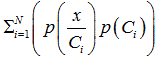 is the posteriori probability that the pattern x belongs to class Ci .
SVM Classifier
SVM is a training algorithm for classification rule from the data set which trains the classifier. it is then used to predict the class of the new sample. SVM is expressed systematically as a weighted combination of kernel functions on training examples. The inner product of two vectors in linear or nonlinear feature space is represented by the kernel function. In a high dimensional space, a SVM creates a hyper plane or set of hyper planes that define decision boundary and point to form the decision boundary between the classes called support vector threat as parameter [37].
ANN Classifier
A neural network model which is the branch of artificial intelligence which teaches the system to execute task, instead of programming computational system to do definite task. It is made up of many artificial neurons which are correlated together in accordance with explicit network architecture. The objective of the neural network receives one or more inputs and sums them to produce an output. Usually, the sums of each node are weighted, and the sum is passed through a function known as an activation or transfer function. The teaching mode can be supervised or unsupervised. ANNs have the potential of solving problems in which some inputs and corresponding output values are known, but the relationship between the inputs and outputs is difficult to translate into a mathematical function. It predicts when pattern is too complex to be noticed by either humans or other computer techniques [38,39]. The most used ANN classifier is feedforward back propagation (B-P).
The Feedforward B-P Algorithm
In order to train the neural network, it cycles through two distinct passes, a forward pass (computation of outputs of all the neurons in the network) followed by a backward pass (propagation of error and adjustment of weights) through the layers of the network. The algorithm alternates between these passes several times as it scans the training data. Thus, with the appropriate combination of training, learning and transfer functions the dataset classification uses the most successful tool called back propagation neural network [38]. The following parameters are considered to measure the efficiency of the network.
The sigmoid logistic function used by standard back-propagation algorithm can be generalized to:
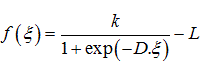 (25)
(25)
Where, K is Kullback-Liebler information distance, learning with logarithmic error metrics was also less prone, the parameter D (sharpness or slope) of the sigmoidal transfer function.
Classifier
The C4.5 can be referred as the statistic classifier. This algorithm uses gain ratio for feature selection and to construct the decision tree. It handles both continuous and discrete features. C4.5 algorithm is widely used because of its quick classification and high precision [37].
Chapter Three Related Work
Introduction
Accurate classification, grading, sorting of foods or agricultural products are needed. It increases the expectations in quality food and safety standards. Thus, computer vision and image processing were nondestructive, accurate and reliable methods to achieve target of classification and grading of sample products.
In this chapter some kinds of concepts were explored by many researchers with different image processing approaches that will be reviewed.
Classification of Coffee
Asma Redi [9] developed raw quality value classification of Ethiopian coffee bean in the case of Wollega region. This research work uses different techniques to remove noise from the sample image. Background subtraction was conducted to avoid blurs, light distortions and other noises that could be formed due to illumination effects and some external objects on the background. Image enhancement and histogram thresholding were used for the extraction of morphological features and color features from the threshold images of the 7 grade levels of Wollega coffee beans. A combined morphological and color features aggregate function dataset were used to develop the classification model. The classification models were built with the Naïve Bayes, C4.5 and ANN yielding a performance of 82.72%, 82.09% and 80.25%, respectively. In order to enhance the classification performance discretization of the dataset into raw quality value into three bean were used. Regression model for the relation between the raw quality values and the combined aggregate feature values of the sample coffee beans were designed to supporting suitability and accuracy of dataset for classification. However, this research work was limited to classification model for raw quality value classification purposes by utilizing smaller number of dataset from each grade level of coffee bean sample.
Quality Assessment of Cereals
Rupali et al [10] demonstrated the classification of wheat grains according to their grades to determine the quality. Acquiring sample image of wheat was with a uniform background which is black color and grains are spread on a black sheet randomly. This research work uses smoothing filtering techniques to enhance images and remove noise. Then, thresholding techniques was used to separate the wheat kernel from the background. They used canny edge detector to detect edges with strong intensity. The various features extracted were color features, morphological features and texture features. The classification models were built with the SVM and Naive Bayes classifiers. To evaluate the classification accuracy, from the total of 1300 data sets 50% were used for training and the remaining 50% were used for testing. Finally, they show the overall accuracy of SVM and Naive Bayes classifier yielding a performance of 94.45% and 92.60%, respectively.
Daniel Hailemichael [11] developed a system capable of assessing the quality of maize sample constituents using digital image processing techniques and ANN classifier based on the standard for maize set by the Quality and Standards Authority of Ethiopia (QSAE). Preprocessing technique was used to remove the false regions. This research work uses various segmentation techniques to separate maize sample constituents from each other and from the background.This component contained three sub-components, namely, color structure tensor segmentation, thresholding and merging. Color structure segmentation algorithm was used to change a copy of the output of the preprocessing component into an image free of shadows, shades and specularities. Thresholding sub-component was used to segments copies of each of the three RGB components. Moreover, thresholding sub-component extracts information from each of the three binary images to form an intermediate image called reconstructed image. The reconstructed image and the color structure tensor segmented image were merged to form an image consisting complete information of the location of pest damage, discoloration and rottenness of maize kernels, called merged image. A merged image contains all the information required to extract the 24 (14 color, 8 shape and 2 size) identified features. The classification components were built with a feedforward ANN classifier with B-P learning algorithm and the class counters sub-components. The system performs that the overall success rate for the classification of maize sample is 97.8%. However, during image acquisition, the maize sample taken was exposed to light; due to this the difference in illumination in a single image affects the values of the color features to be extracted, and introduces shadows and shadings.
Abirami et al [12] developed analysis of rice granules using image processing techniques and ANN classifier. The research uses image analysis techniques to remove noise from the sample image using median filters. Adaptive threshold was implemented to detach the regions in an image with reverence to the stuffs. This partition was based on the discrepancy of intensity between the object pixels and the background pixels. Sobel edge detector is used to distinguish the edges by locating the local maxima and minima of the gradient of the intensity function. The features which were extracted from images of rice kernels are perimeter, area, minor-axis length and major-axis length using contour detection. This work claimed that when there is no overlap of grains, the system is able to classify well for all the grains and the accuracy was found to be 98.7%.
Grading of Fruits
- [13], developed a novel technique for grading of dates using shape and texture feature. The system removed the specular reflection and small noise using a median filter. Threshold based segmentation was performed for background removal and fruit part selection from the given image. Curvelet transform and local binary pattern were employed to extract shape features using the contour of the date fruit and texture features are extracted from the selected date fruit region. The combinations of shape and texture features were fused to grade the dates into six grades. Classifiers such as K-Means and SVM were used. The system yields best grading accuracy of 96.45% with error rate of 3.55%.
Classification of Oil Seeds
- [14] developed classification of olive oil seeds using ANN classifier. The system uses five different olive oil types to characterize the features from the sample image. Chemo metrical procedure and absorbance at pre-selected optimal wavelengths were used. A stepwise selection procedure in linear discriminant analysis was conducted to choose wavelengths in the olive oil type. ANN were used for classification of the oil and yielding a performance of 98%.
Summary
We reviewed related works on automatic classification and grading of agricultural products using digital image processing techniques. It was pointed out that various techniques have been proposed over the years to automate classification and grading of agricultural products. Literature reveals that the proposed techniques depend on the type of the agricultural product. Thus, a system developed for classification and grading of agricultural product could not be directly applied for other products. Thus, in this thesis, we propose an automatic classification and grading system for Ethiopian sesame grains.
Chapter Four Design for Sesame Grain Classification and Grading System
Introduction
This chapter presents, the details about the proposed system architecture, image processing techniques such as the process of sampling and representativeness of sesame grain. How the sample image is preprocessed for further analysis, the segmentation techniques to isolate background from foreground and separate touched sample sesame grains and the extracted features from the segmented image used in this study are also briefly presented. This is then followed by giving a brief explanation on the generalized model used for classification and grading of sesame grain.
The Proposed System Architecture
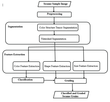
Our proposed grading system is a system which loads image of sesame grains, preprocesses the image, detect the edges of sesame grain samples, extracts proper image features i.e., morphological and color features then classifies sesame grains into their respective origin based on their growing regions and finally, grade the classified sesame grains into their distinct grade levels using the extracted image features. The proposed system architecture has six components, namely: image acquisition, preprocessing, segmentation, feature extraction, classification and grading model. Given sesame grain samples, images are preprocessed to remove noise. The preliminary task to prepare the image for next phase which is segmentation is also done here. The segmentation stage is responsible for accomplish the work of partitioning sesame grain’s region and other constituents on the image. Two different segmentation techniques are applied for proper separation of sesame grains from other constituents and background of the image. The segmented image contains all the attributes necessary for feature extraction. The next stage of the proposed architecture is feature extraction. This is carried out by extracting all the required features, such as size, shape, and color, of the sesame grain sample. These extracted features will be serve as input for classification and grading stage.
For this research, the classification is performed mainly based on color attribute of extracted image. The grading process is performed by examining the remaining two attributes, size, and shape of the extracted sample image. Figure 4.1 represents the proposed system architecture.
Figure 4.1: Proposed System Architecture
Sesame Sample Image
Image acquisition process is the predominant class of image processing technique. All images used for this research are captured inside the warehouses of the ECX, in Addis Ababa and Humera. The classes and grade levels of each sesame grain sample used for this work were certified by the domain experts who are currently working in the ECX’s laboratory. Sesame grains grown around these four regions, namely Bale, Jawi, Assosa and Kemissie, are sampled and processed independently inside the ECX laboratory. They are generally categorized under Wollega Sesame. The sesame grains grown in Gonder, Combolicha, Kafta Humera, Setit Humera, Wolkait, Metema and Quara are categorized under Humera sesame. Their grading process is also done in similar fashion as that of Wollega sesame in the second warehouse of ECX found in Humera. The grading parameters which are used in both warehouses are identical in all rounds. All sampled sesame grain were the products of 2007/08 EC production year. The samples have been taken from May 10th up to July 30th 2009 EC.
For this study, the collected sample images of sesame were taken with Sonny VIXIA HF M50 HD camera with a resolution of 4288×2848. The distance between the sample and the camera is 14cm, the view of the camera is 10cm×15cm, the camera focuses at the center of the field view vertically downward and in JPEG file format.
Moreover, the selection of background object should contrast the region of interest. In this research, we were used different background colors such as black, pink, brown, green and cyan. Among them, cyan were highly contrasts than others. After selection of background object, the samples were distributed randomly on the selected background object. In digital image processing weight is equivalent to area of the object. Thus, the volume of samples for all grades should be in an equal weight. A total of 750 images were taken from the two regions, Humera and Wollega. Some of sample sesame images are depicted in Annex B.
Preprocessing
The exactness of classification, grading and sorting of agricultural products models mainly depends on the preprocessing process. The raw data is subjected to several preliminary processing steps to make it functional in the descriptive stages of sesame grading. In order to get sesame grain features accurately, sesame grain images are preprocessed through different preprocessing methods. The result of these stages will apply to the next stage, segmentation.
In view of this, noise removal preprocessing algorithm was used. First, for each of these techniques the images were converted into gray scale image. The noise induced during image acquisition is removed using median filtering. One of the main goals of preprocessing is removing the noise by reserving the edges. Thus, median filtering is quite widely used in this thesis because, under certain conditions, it preserves edges while removing noise. This how it works, the acquired image is converted to gray image then the median filtering algorithm simply run through the pixel entry by entry, replacing each entry with the median of neighboring entries.
The sample sesame grain image, before the implementation of median filtering and its equivalent image after median filter applied are shown in Figure 4.2(a),(b), respectively.
Figure 4.2: (a) The Gray Image (b) Median Filtered Image
Segmentation
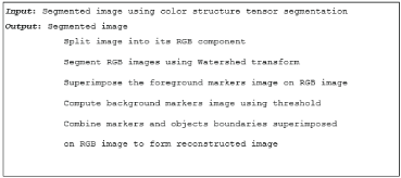
No single standard method of image segmentation has emerged. Rather, there are collections of ad hoc methods that have received some degree of popularity. To tackle the task on hand, we came up with two segmentation technique for proper classification and grading of sesame grain. The proposed segmentation algorithms are color structural tensor and classical watershed transform segmentation. To the best of our knowledge, these algorithms are new and never been used in other researches. Applying color structure tensor segmentation for rendering better result is not an appropriate method. As we can see from the original sample sesame image one can easily observe that there are so many connected objects. This can be sesame-sesame, sesame-foreign particle, or both. As a result, a segmentation method other than color structure tensor is needed. Classical watershed transform segmentation is used to separate the connected objects by avoiding the over segmentation drawbacks with the former, the ordinary watershed segmentation. The general over view algorithm for proposed segmentation process is depicted in Algorithm 4.1.
Algorithm 4.1: Result of Segmentation
Color Structure Tensor Segmentation
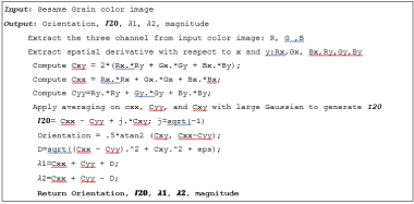
Color structure tensor segmentation, adequately handles the vector nature of color images. It models the linear structure and to measure the local color symmetry in a color image. Further, since color structure tensor supports dichromatic reflection model, we combine the features based on the color tensor with photometric invariant derivatives. These photometric invariant derivatives are incorporated in the color tensor, hereby allowing the computation of dichromatic shadow-shading quasi-invariant model. The dichromatic model divides the refection in the interface (specular) and body (diffuse) refection component for optically inhomogeneous materials. The combination of the photometric invariance theory and color structure tensor based segmentation removes shadows and specularities introduced in an image through amplifying the interest of an object. Moreover, color structure tensor can be implemented by filtering of the orientation tensor. Therefore, this activity is employed as preprocessing due to its capability to suppress noise in color images. Eigenvalues λ2 and λ1 are represented by amplifier regions low linear strength and high linear strength, respectively. On the other hand, the difference in the two eigenvalues will be used to enhance the line energy in each pixel. Algorithm 4.2 computes ????????????, orientation, magnitude and eigenvalues according to Equation 16 to Equation 20.
Algorithm 4.2: Computation of ????????????, Orientation, Magnitude and Eigenvalues
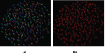
The result obtained from color structure and comparison made between the two eigenvalues where (a) is the original image, (b) is the first eigenvalue, (c) is the second eigenvalue are shown in Figure 4.4.
Figure 4.4: Sample of Sesame Grain and its Color Structure Tensor in RGB Color Space.
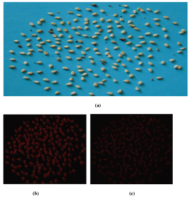
As we can see from Figure 4.4, the resultant image of the two eigenvalues λ1 and λ2 amplify noise, shadows and specularity. Color structure tensor output image is called ????20. ????20 is a complex or vector image which has two information: magnitude (holds the linear strength) and direction (holds the color information).
Hence, color structure tensor models the linear strength, removal of noises, the dichromatic shadow shading quasi-invariant and thresholding operations will be done on ????20 and its magnitude. Figure 4.5 presents the result I20 complex image sample sesame grain image and its magnitude.
Figure 4.5: (a) The Result of Complex ????20 in RGB (b) Magnitude of ????20 in RGB
Equivalently, noise introduced in ????20 can be suppressed by applying pixel-wise operation as follows:
![]() (26)
(26)
Where, ????20 has been computed from Equation (18) and, λ1 and λ2 represents the eigenvalues computed from Equation (14) and Equation (15), respectively. Moreover, shadows and specularities are removed using the best feature dichromatic reflection model, shadow shading quasi-invariant method.
Pseudo code generation to suppress noise introduced in the above scenario is presented in Algorithm 4.3.
Algorithm 4.3: Preprocessing Image Using Color Structure Tensor.
Figure 4.6 shows the result of complex ????20 and its magnitude obtained after suppressing noise introduced by lowest eigenvalues, free from shadow effects.
Figure 4.6: (a) ????20 after Suppressing Noise (b) Magnitude Information
The next step is thresholding the image using color structure tensor thresholding method. Color structure tensor segmentation is used to remove unpredictable objects and amplifies the object of interest. Before we get the proper threshold value, we have applied normalization techniques with constant values to isolate foreground from background object. This helps to select the best threshold value on the magnitude of ????20. After color structure tensor threshold is applied, further morphological filling followed by removal of tiny objects using morphological erosion operation and filling holes are crucial steps to reveal a better result. Algorithm 4.4 shows the pseudo code for segmentation of foreground object from background.
Algorithm 4.4: Isolation of Foreground object from Background
Figure 4.7 presents the result of color structure tensor thresholding after a series of morphological operations done and showing the detail information of sesame grain and foreign particles.
Figure 4.7: Result of Segmentation Using Color Structure Tensor.
Watershed Segmentation
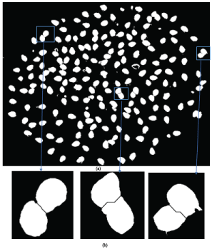
The goal of watershed segmentation is to present numerical tests for the segmentation problem using mathematical morphology tools. The approach used in this work is based on the classical watershed transform segmentation. Since the sample sesame grains are distributed randomly there will be an overlapping of objects. Thus, this segmentation method is more applicable when touched objects are found in a given image. However, the former watershed algorithm gives an over segmentation and to avoid this drawback, a marker technique can be used. We have considered the color structure tensor threshold image as an input for this segmentation. The over segmentation is clearly seen and corrected by applying a morphological filter.
However, as the over segmentation is due to the fact that we obtain a lot of minima, and the use of morphological filters can only suppress some of them, then another way to act on these minima is to apply the swamping approach, by imposing markers for the new minima. Clearly, the number of minima is attenuated. To obtain the wanted final contours which are derived from the watershed of the gradient modulus, we have to compute the watershed of the swamping of the gradient modulus of the filtered image.
Moreover, the classical watershed transform method uses the sobel edge detector to detect the gradient magnitude and regions obtained which will be used as markers. This result will be useful in discrimination of sesame grain from foreign matter particles. From the comparison, Sobel operator is selected since it gives more sharp and clear edges as compared to other operators and smoothing effect is attractive and create a difference in objects. In order to gain the boundaries of the segmented image, we used morphological operator such as erosion and dilation.
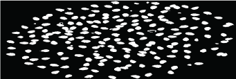
In Figure 4.8 (a) shows the result of segmented image using classical watershed transform segmentation and (b) the corresponding segmented sample image of individual objects.
Figure 4.8:Result of Segmentation Using Watershed
Feature Extraction
Image analysis is the process of extracting meaningful information from images. Feature extraction process in our study is responsible for extracting the essential attributes from sample sesame grain. Thus, the most important features used to classify and grade sesame grain are color, size and shape features gained from both color structure tensor and classical watershed transform segmentation. The next subsections present all the color, size and shape features extracted from sesame grain sample.
Color Feature Extraction
Color is an important feature for image representation. The color features for this work were extracted using RGB and L*a*b* color space model from the color image of color structure tensor threshold. The human color perception is quite subjective as regarding perceptual similarity. As a result, colors of the RGB space are usually not easy for humans to interpret. However, the L*a*b* color space model describes in the most complete way all the visually perceived colors and very applicable in identifying color differences between objects. For instance, the color of whitish Humera, whitish Wollega and reddish Wollega sesame grain is different. Therefore, the color features are extracted by computing the mean values of RGB and L*a*b* of sesame grain images. The first set of features, is the mean values of the red, green, and blue components of each image as computed from its three color channel functions using Equation (2).
The second set of color features measured in this work is based on the L*a*b* color space model. L*a*b* color model color is described by three components: Luminance or brightness is an attribute of the L channel which has values ranging from 0 up to 100 which corresponds to different shades from black to white. The a* channel has values ranging from −128 up to +127 and gives the red to green ratio. The b* channel also has values ranging from −128 up to +127 and gives the yellow to blue ratio. Thus, a high value in a* or b* channel represents a color having more red or yellow and a low value represents a color having more green or blue. Since the sesame regions are bright and less illuminated than the surroundings, it is easy to locate them in the L channel since the L channel holds lightness information. The a* and b* channel values are also lesser in the sesame areas.
In this research work, the color features are extracted using the mean values of each component of the L*a*b* model and are calculated for each foreground region by using Equation 7-9. A total of six color features have been selected to represent the color features of sample sesame grain images.
Size Feature Extraction
Morphology is the geometric property of images. In our case, it is the size and shape characteristics of sesame grains. This research work uses only area size features to determine the area of sesame grain and the foreign matters. Because of area is the number of pixels inside the region covered by sesame grain or foreign matter, including the boundary region will be detected. After, the necessary image transformations is made over the RGB image of the sesame grain, the edges of the sesame and the foreign matter are marked as pixel over the image. Thus, area of the edge detected sesame and foreign matter provides information about the actual size.
Shape Feature Extraction
In this study, the discrimination power obtained from the size feature extracted were not enough to describe the actual difference between the sesame grain and the foreign matter. As a result, a descriptor other than size is needed. Thus, shape of an object is an important and basic visual feature for describing image content. Shape descriptors are used to give numerical results with respect to the shape property of an object. Therefore, it is the second helpful descriptor to differentiate the sesame grain from foreign matters. In this approach, we used three shape metrics major axis length, minor axis length and eccentricity. These features are computed from the binary image of each objects. After we have extracted those 10 features, we used each feature for the identification separately as an input to the classification and grading model.
Classification
Though classification has been used broadly over years, classifiers modeled for various agricultural products could not be applied for the classification of sesame grains. Thus, we have developed rule based classification approach using color difference algorithm, called delta E classifier. The classification process is fully dependent on the extracted color features from each predefined classes of the sesame grain. The proposed approach for classification process consists of K cluster centroids representing L*a*b* color triplets. All of the color information is in the 'a*' and 'b*' layers. We can measure the difference between two colors using the Euclidean distance metric using Equation 11.
The difference between two color samples is often expressed as delta E. This can be used in the classification to show whether a testing sample is in tolerance with a reference samples of different types of sesame grains. The color difference between the L*, a* and b* values of the references and the test image will be computed. The resulting delta E number provides the required information that enables to decide how close or similar two color sampled images are in a color space. For our research, we used four images as an input for the classifier. Out of these, three of them are known standard images namely: whitish Humera, whitish Wollega and reddish Wollega sesame and the other one is a test image. Based on Equation 11, the delta E difference has been computed for each L*, a* and b* color space. The three standard images will find their color difference from the test image using the delta value of the three-color channels. The smaller delta value will determine the class of the given test image. The entire process is shown in Algorithm 4.5.
Algorithm 4.5: Steps of Delta E Classifier
Figure 4.9 (a) shows the test image (b) shows the respective L* values (c) shows a* values and (d) shows b* values.
Figure 4.9:(a) Input Test Image (b) Luminance Value (c) a* Value (d) b* Value
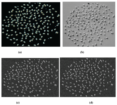
Grading
The proposed grading approach is based on the grading rules implemented in the ECX. Once the image is segmented, the next step is feature extraction. Based on inspection of the sesame grain, size (e.g., area) and shape (e.g.; eccentricity, centroid, minor and major axis) are the two attributes that contain efficient information to discriminate sesame grain from foreign matter.
Thus, to differentiate sesame grains from the foreign particle, the system or grading algorithm set to learn the area of sesame grains. Once the system get used to the area of sesame grain, area is used as a primitive way of identifying the sesame grains. For example, in our case, the area of the sesame grain lies between 300-500, i.e., any object which has an area out of this range can be categorized as foreign particle. However, there are foreign particles where areas lie in that range. Thus, to point out the sesame grains only, it was necessary to consider other attributes too, like shape feature. Among different categories of shape features, we here used the minor axis, major axis, and eccentricity as a shape feature for the intended task. By using a region props function, we could be able to get the required features easily. These features are most of the time unique. This means the sesame grain has a specific range of minor axis, major axis, and eccentric value. For example, the minor axis, major axis, and eccentric of an extracted sesame grain is 30-45, 70-85 and 0.8, respectively. At this point, we have two isolated regions, one region only containing sesame grains and the other containing foreign particles. But to proceed from here, it was needed to come up with a different way of conducting the grading. This is why the idea of calibration is used. Calibration “Calibration in measurement technology is the comparison of measurement values delivered by a device under test with those of a calibration standard of known accuracy.” Thus, to calibrate the grading system, we used different sample images with already known grade levels and this in depicted in Annex C. The grading system is performed using the following steps.
- The sesame grains are separated from the foreign particles using size and shape features.
- Total area of the sesame grains is computed.
- Total area of the foreign particles is computed.
- The ratio of total area of the foreign particles to total area of the sesame grains is computed and for our purpose, we named it, “weight”.
- The weight value labeled is with the corresponding grading level
We identified the weight range values through empirical analysis. Based on the weight value, the sampled sesame grain is grouped into one of different grade levels. The overall rule based grading system and its implementation is presented in Annex A. The numeric range values from the calibration process for Humera and Wollega type sesame grain grades are shown in Table 4.1.
Table 4.1: Weight Range Values of Sesame Grains
|
Grades |
Weight Values |
||
|
Whitish Humera |
Whitish Wollega |
Reddish Wollega |
|
|
1 |
0-0.2 |
0.1-0.3 |
0-0.1 |
|
2 |
0.3-0.6 | 0.3-0.5 | 0.2-0.4 |
|
3 |
0.6-0.8 | 0.6-0.7 | 0.5-0.7 |
|
4 |
0.8-1.0 | 0.7-0.8 | 0.8-1.0 |
|
5 |
____ |
0.85-1.0 |
____ |
|
Under Grade |
Above 1.0 |
Above 1.0 |
Above 1.0 |
Chapter Five Experiment
Introduction
In this study, an attempt is made to test the effectiveness of our proposed system design. This is an integral part of the design and give an indication how the system will perform. Moreover, it also provides a platform to assess its strength and weakness. The data set used to conduct the tests the implementation procedure, results obtained from both classification and grading and comparison against the manual system will be discussed in detail.
Dataset Preparation
Since there is no readymade dataset for this type of research, we have prepared our own dataset to evaluate the performance. To do so, sesame grains have been collected from the ECX warehouses. The collected sesame grains are certified by the domain experts who work in the ECX laboratories. A total of 750 images are captured for calibrating and testing the proposed model. The data were partitioned randomly into calibrate, validation and test sets. Image acquisition is done using a Sonny VIXIA HF M50 HD with a resolution of 4288×2848. The distance between the sample and the camera is 14 cm, the view of the camera is 10cm×15cm. The camera focus is mounted on a stand at the center of this field view vertically downward and the file format is JPEG. Moreover, the selected background color was cyan.
For classification, 70% of the data is used for validation or as standard images and the rest are used for testing. The 70% equally shared whitish Humera type, whitish Wollega type and reddish Wollega sesame type. The data were partitioned randomly into standard and test sets. Similarly, for grading, 40% of the data is used to calibrate the system which is to get weighting scale of each grade level and 30% of the data is used for validation. The rest of the data is used for testing. The calibration data set is used to find the absolute numerical range of each grade level, i.e., getting the range of weighting scale of each grade level by calculating the ratio of the sum of total area of the foreign particles to sesame grains. The test data set is used to evaluate the performance of the proposed grading system. In our experimentation, we used 225 (45 for each grades) test images of the data set.
Implementation
The system prototype is developed with MATLAB tool with version R2010a. The computer on which the system is implemented is Intel® core™ i5 with 6GB RAM and 2.67 GHz processor. The graphical user interface of the developed prototype is shown in Figure 5.1.
Figure 5.1: Graphical User Interface of the Developed Prototype.
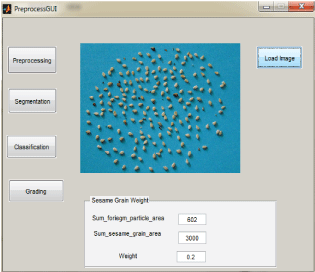
Experimental Results
Once the automated rule-based model is developed, consecutive experiments are conducted to assess the intended purpose of the proposed model, classification and grading of sesame grain. To this end, experiments are carried out to classify the sesame grains based on their color attributes and grade them to their respective grading level based on their morphology features. Furthermore, a comparison between the proposed classification and grading model and existing classification is performed to evaluate the performance and accuracy of the former one.
Performance Evaluation
Performance evaluation of classification model is important for understanding the quality of the model, to refine the model and for choosing the adequate model. The confusion matrix displays the number of correct and incorrect predictions made by the model compared with the actual classifications in the test data [40]. Confusion matrix for a classifier with two classes true and false is presented in Table 5.1.
Table 5.1: The Confusion Matrix of a Classifier with Two Classes.
|
Classes Predicted
Current Classes
|
True Class |
False Class |
|
True Class |
True Positive |
False Positive |
|
False Class |
True Negative |
False Negative |
The number of correctly predicted values relative to the total number of predicted values is specified by precision parameter that takes values between 0 and 1. Precision equal to 0 indicates that the model has no predictive power and not conclusive [40] and precision equal to 1 indicates both predictive power & conclusive. Evaluation of the classification and grading algorithms are one of the key points in any digital image processing. The performance evaluation metrics commonly used in analyzing the results of classification algorithms applied are accuracy measure and error measurement using relative error (mean percentage error) propagation [40]. The accuracy is the proportion of the total number of correct predictions and calculated as the ratio between the number of cases correctly classified and the total number of cases [40].
 (27)
(27)
Where, P: positives which refer to the total number of positive tuples.
N: negatives which refer the total number of negative tuples.
TP: True positives which refer positive tuples that were correctly labeled by classifier.
TN: True negatives which refer negative tuples that were correctly labeled by classifier.
FP: False positives which refer the negative tuples that were mislabeled as positive.
FN: False negatives which refer the positive tuples that were mislabeled as negative.
The Error indicates the proportion of cases classified incorrectly.
![]() (28)
(28)
Where, accuracy is the proportion of the total number of correct predictions.
The mean percentage error or relative error (MRE) is computed using below:
 (29)
(29)
Where, n represents the number of samples, represents the ith automatically measured value in the ith input image and represents the ith manually measured value in the ith input image.
Classification: The classification algorithm for the proposed model is based on the mathematical calculation of standard delta E, color difference algorithm. In this experiment, the six color features are used as input to the classifier. There were also three output classes that correspond to the three-predefined sesame growing regions. Once the sampled image is classified into its respective region of growing, accuracy checkup will follow for validation. This is mostly performed by comparing it with the result we got from the manual procedure or traditional way of classification. The performance of delta E classifier was tested with 225 (30% of data set) test images, i.e., 75 test images for each class. Table 5.2 shows the confusion matrix for the accuracy of classification.
Table 5.2: Confusion Matrix for Accuracy of Classification.
|
Actual Class
Predicted Class |
Whitish Humera |
Whitish Wollega |
Reddish Wollega |
|
Whitish Humera |
89.3% | 9.3% | 0.0% |
|
Whitish Wollega |
23.0% | 75.0% | 0.0% |
|
Reddish Wollega |
0.0% | 0.0% | 100.0% |
|
Accuracy%
|
88.2% | ||
Table 5.2 reveals the number of sample images that is correctly classified and misclassified for each class. The elements of the table show the number of test examples whose actual class was the row heading and whose predicted class was the column heading. The diagonal elements show instances that were correctly classified. Other elements showed misclassified instances in relation to the corresponding row and column labels. In general, the overall classification of delta E classifier on the selected color feature is calculated using equation 27 and 28. Results show that from the total test examples of 225 instances, 208(88.2 %) were correctly classified and 17 (11.8 %) were misclassified. In consideration of this, whitish Humera sesame was misclassified more to whitish Wollega sesame and whitish Wollega sesame was more misclassified to whitish Humera sesame. This shows that there is a strong color relationship between the whitish Humera and whitish Wollega sesame grains.
A closer look at the color structure of these sesame grains shows their relative closer color than from reddish Wollega sesame. Here, we experienced a systematical error of 11.8 which might originate from the quality of the camera itself. Since both the whitish Humera and whitish Wollega sesame have similar color, white, sometime it is difficult to capture an image with high resolution. An investigation of the results indicated that, the color segmentation approach we used in this work obtained permissible result for classification of the sesame grains with some limitations.
Segmentation Result of Sesame Grain and Foreign Matter
The accuracy of a given system in image processing mainly relies on the segmentation techniques used. Identifying sesame grain and foreign particles in the automated proposed algorithm as well as in manual work is done through the help of size and shape features. In contrast to this, since manual segmentation is done using experts in tedious way it is exposed to errors. Therefore, this result will introduce pitfalls in next step weighting of the sesame grains and foreign particles with weight scale separately since the experts who identify the sesame and foreign particle are easily get tired. This in turn leads to giving wrong grade levels.
The method we proposed in this work reaches out those problems through automated segmentation and identifying techniques. For this experiment, we selected five images from five grade levels of Humera sesame grain to investigate how the discrimination power resulted from the proposed segmentation technique and the corresponding identifying in manual system. Hence, our ground true value is based on free from any error in identification of sesame and foreign matters. Thus, to make it more realistic and more prone to error, the same image is analyzed by the crew of ECX laboratory technicians and using the proposed discrimination algorithm. The average result was considered as a good measure for making comparison between manual and automated computation against to the ground truth.
Sample images along with identification of sesame and foreign particles and weighing process are shown in the Annex A. A total of 225 (30% of data set), i.e., 45 data set are used for each grade. As shown in Table 5.3, the proposed algorithm for identification of sample images of sesame grain and foreign matters are compared relative to manually computed result.
Table 5.3: Test Result of Sample Images.
|
Number of Images |
Sample Image |
MI for sesame |
MI for foreign matter |
PI for sesame |
PI for foreign matter |
GT for IS |
GT for IFM |
Relative error in MI for sesame % |
Relative error in MI for foreign matter % |
Relative error in PI for sesame % |
Relative error in PI for foreign matter % |
|
1 |
HSG1 |
27 |
18 |
37 |
9 |
0 |
0 |
10 |
9 |
2 |
2 |
|
2 |
HSG2 |
25 |
20 |
29 |
16 |
0 |
0 |
4 |
4 |
7 |
4 |
|
3 |
HSG3 |
21 |
14 |
30 |
17 |
0 |
0 |
9 |
3 |
1 |
3 |
|
4 |
HSG4 |
17 |
28 |
19 |
27 |
0 |
0 |
2 |
1 |
7 |
5 |
|
5 |
HSUG |
14 |
31 |
12 |
33 |
0 |
0 |
2 |
2 |
3 |
2 |
|
Mean Error (%) |
5.4 | 3.8 | 4.0 | 3.4 | |||||||
Where, GT, IS, IFM MI and PI stands for ground truth, identification of sesame, identification of foreign matters, manual identification and proposed algorithm identification, respectively. Furthermore, the identifying error is the proportion of the difference between the numbers of proposed algorithm identified instances, regardless of true or false results, to the true number of instances with that of obtained using manual identification.
In view of this result, the measuring mean percentage error of number of identified sesame is calculated using Equation 29. The measuring mean percentage error for sesame using the proposed algorithm is 4.0; whereas the measuring mean absolute error for identified of foreign matters using the proposed algorithm is 3.4. On the other hand, the measuring mean percentage error for sesame using the proposed algorithm is 5.4; whereas the measuring mean absolute error for identified of foreign matters using the proposed algorithm is 3.8. Clearly, the relative error in the proposed identification algorithm is considerably lesser than the manual work. Figure 5.2 presents error comparison between the identification algorithm for the proposed and manual systems.
Figure 5.2: Error Propagation in Identifying Sesame Grains and Foreign Particles
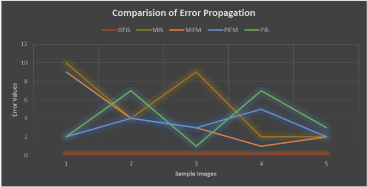
Grading
The performance of the automated grading system of sesame grain is evaluated with respect to the manual grading approach. The size and shape features are used to differentiate sesame grains from the foreign matters. The discrimination power of both features using the proposed segmentation approach will be examined in the next section.
For testing purpose, we only considered the Humera type sesame which has five grade levels. Once we got the corresponding “weight” value of each grade levels using the calibration process, the absolute numerical range for each grade levels were set accordingly. For example, if the test input image is grade one Humera sesame, weight ratio value should be within 0-0.2. Therefore, from the data set 225 (30%) of test data will be used. Among those, test data sets we divide into five grades i.e., 45 items for each grade level. Thus, five output grades that correspond to the five predefined Humera sesame grain will be expected.
Table 5.4-5.6 show confusion matrix for accuracy of proposed sesame grading system using grades from whitish Humera sesame grain, whitish Wollega and reddish Wollega. Where:
Table 5.4: Confusion Matrix for Accuracy of Grading System of Whitish Humera Sesame
|
Actual Grade
Predicted Grade |
WHG1 |
WHG2 |
WHG3 |
WHG4 |
WHUG |
|
WHG1 |
97.7% | 2.2% | 0.0% | 0.0% | 0.0% |
|
WHG2 |
0.0% | 97.7% | 2.2% | 0.0% | 0.0% |
|
WHG3 |
0.0% | 0.0% | 97.7% | 2.2% | 0.0% |
|
WHG4 |
0.0% | 0.0% | 0.0% | 84.4% | 15.5% |
|
WHUG |
0.0% | 0.0% | 0.0% | 20.2% | 75.7% |
|
Accuracy% |
92.04% | ||||
Table 5.5: Confusion Matrix for Accuracy of Grading System of Whitish Wollega Sesame
|
Actual Grade
Predicted Grade |
WWG1 |
WWG2 |
WWG3 |
WWG4 |
WWG5 |
WWUG |
|
WWG1 |
97.7% | 2.2% | 0.0% | 0.0% | 0.0% | 0.0% |
|
WWG2 |
2.2% |
97.7% |
0.0% | 0.0% | 0.0% | 0.0% |
|
WWG3 |
0.0% | 0.0% | 100.0% | 0.0% | 0.0% | 0.0% |
|
WWG4 |
0.0% | 0.0% | 0.0% | 95.5% | 0.0% | 0.0% |
|
WWG5 |
0.0% | 0.0% | 0.0% | 0.0% | 95.5% | 4.4% |
|
WWUG |
0.0% | 0.0% | 0.0% | 0.0% | 4.4% | 95.5% |
|
Accuracy% |
95.35 | |||||
Table 5.6: Confusion Matrix for Accuracy of Grading System of Reddish Humera Sesame
|
Actual Grade
Predicted grade |
RWG1 |
RWG2 |
RWG3 |
RWG4 |
RWUG |
|
RWG1 |
100.0% | 0.0% | 0.0% | 0.0% | 0.0% |
|
RWG2 |
0.0% | 100.0% | 0.0% | 0.0% | 0.0% |
|
RWG3 |
0.0% | 0.0% | 100.0% | 0.0% | 0.0% |
|
RWG4 |
0.0% | 0.0% | 0.0% | 95.5% | 4.2% |
|
RWUG |
0.0% | 0.0% | 0.0% | 4.4% | 95.5% |
|
Accuracy% |
94.4% |
||||
•WHG1, WHG2, WHG3, WHG4 and WHUG stands for grade one, grade two, grade three, grade four and under grade of whitish Humera sesame, respectively.
•WWG1, WWG2, WWG3, WWG4, WWG5 and WWUG stands for grade one, grade two, grade three, grade four, grade five and under grade of whitish Wollega sesame, respectively.
•WRG1, WRG2, WRG3, WRG4 and WRUG stands for grade one, grade two, grade three, grade four and under grade of reddish Wollega sesame, respectively.
Based on this experimental result, we have computed the overall accuracy and the error propagation using Equation 27 and 28. Out of 225 images, the overall grading accuracy, 93.3% were correctly graded and 6.7% of the sample data set images was incorrectly graded. An investigation of the results indicated that one image in each of grades were incorrectly classified as other than their respective grades. In addition, except under grade class all the images of grade one, two, three and four varieties are perfectly graded. As we can see, here also we experienced very few systematic error which is highly related with the last two grade levels of distinct sesame grain varieties. The last grade levels have almost the same constituents of foreign particles. This makes the grading more complex because our grading algorithm mainly relies on the area of foreign particles.
The other criterion area of comparison of performance between our proposed systems against the manual system is based on the time taken to perform the same function. In order to do that, first, the comparison is done by taking with same sample sesame grains and the classification and grading process was performed using the ECX experts. The time taken by the classification process is much better than the grading. The average time taken for classification and grading of sample sesame grains are 20 minutes. Afterwards, our proposed system takes sample sesame grain images and processed using the proposed digital image processing techniques. The time taken to finish the classification and grading of a given sample image is 56 seconds.
Discussion
The overall experimental evaluation, conducted through the performance measure of sesame grain classification and grading system shows good result. As we can see, the immediate input fed into our proposed grading algorithm is the result of grading of sesame grain into distinct group. Though, human visual inspection is invaluable in determining the class of sesame grain, false estimations might also occur as bias on or loosing concentration are the natural behavior of human being.
Our algorithm to classify and grade sesame grains was tested using sample data selected from the dataset. We applied empirical approach to test the performance of the proposed system. On top of that, comparison of the proposed automated approach has performed better with respect to the manual system. For the classification, our proposed delta E classifier using the color features of each predefined classes is used to enhance the accuracy. As can be seen in Table 5.2, the performance of sesame grain classification model achieved 88.2%, which is a promising result.
Regarding identification of sesame grain and foreign matters, 5 images were tested to check the identification performance. An error measure was used to check the accuracy of the proposed identification algorithm. The mean percentage error to differentiating sesame grain and foreign matter in proposed algorithm is 4.0 and 3.4, respectively. Whereas mean percentage error to differentiating sesame grain and foreign matter in manual system is 5.4 and 3.8, respectively. The performance of sesame grain grading system is also depicted in Table 5.3. From the result, the overall grading accuracy was 93.3 %. Out of the total 225 images (45 samples for each grades) used, only 7 were falsely graded.
However, the lack of proper laboratory settings for image acquisition and imaging factors were some of the challenges reflected on the classification and grading of the sesame grains. The other major issue is segmentation error, an error that occurred due to the segmentation algorithm while the number of touched sesame grains increased the identification error is occurred due to morphological similarities (similarities occurred due to the size and shape features between the sesame grain and foreign matters). Moreover, the calibration process we have used for computing mean weight values for each predefined grades from the three types of sesame grains were time consuming and tedious. The final issue of this work is due to lack of data for the grading of mixed classes of sesame grain, we excluded this class from the research.
Chapter Six Conclusion and Future Work
Conclusion
Sesame is a commercial commodity that plays a major role in earning foreign currency among export commodities of Ethiopia. Countries including Ethiopia produce sesame both for domestic and export consumptions. The grain is used as oil and food item around the world. Sesame grains with those usage is graded by well-equipped laboratories and highly skilled experts using standard parameters set by the ECX. The standard is based on morphological and chemical characteristics of sesame.
Consequently, even if the experts are highly skilled, they may get tired and exposed to bias. As far as the researcher’s knowledge, is concerned no effort has been made by research to support the grading process of Ethiopian sesame grains. In this study, an attempt has been made to construct a model for the classification and grading of Ethiopian sesame grain varieties. In this research work, a segmentation algorithm is developed to recognize the class as well as the grade level of sesame grains. A total of 10 features are identified to model the classes and grade levels of sesame sample.
Classification is performed mainly based on the extracted color attributes of the sample image. Since the colors of whitish Humera and whitish Wollega have similarities in color, the standard delta E color difference algorithm with the 6 color features and 3 output classes is designed. The grading process is performed by examining the remaining two attributes, size, and shape of the extracted sample image. Rule-based grading approach using the weight ratio of foreign matter to sesame grain which is currently employed in the manual system is used. Dealing with this, the total number of sesame grain and foreign matter is identified from the segmented image using the extracted morphological features.
After identification is done the sum of foreign matters will be divided by sum of sesame grains, called weight ratio. The weight value will determine the grade level of the given sample using a specified grade range values. The performance of the proposed system is compared against the manual system currently used by the ECX. Results show that the overall success rate for the classification and grading of sesame sample is 88.2% and 93.3%, respectively. Mean percentage error of segmentation of sesame and foreign particles of the proposed algorithm is 4.0 and 4.2, respectively. Whereas mean percentage error to differentiating sesame grain and foreign matter in manual system is 5.4 and 3.8, respectively. The experts have taken 20 minutes for classification and grading a given sample. However, our proposed system completed the job within 56 seconds which is a promising result against the manual system.
Moreover, the majority of the classification and grading errors are attributed to the challenges faced by the image acquisition and other imaging factors, segmentation and noise removal techniques from non-uniform size sesame grain and foreign matter images, which led to have poor features during feature extraction. As one can see from the result, this study achieves promising result towards classification and grading of sesame grain varieties. We strongly recommend the ECX should replace the old manual system with automated classification and grading system.
Contribution of the Thesis
As a contribution to the new knowledge, this research work has contributed the following.
•We proposed system architecture for the classification and grading of sample sesame grains.
•A preprocessing algorithm to remove noise introduced in sample sesame images is proposed. This algorithm will be applicable for other cereals and agricultural products.
•We proposed a segmentation algorithm that is used to isolate sesame grains from the background and separate the connected sesame grains.
•A classifier is proposed using the color difference between the sample sesame varieties.
•We proposed calibration process to identify the 6 morphological features of sesame sample images.
•We proposed a rule based grading of sesame sample images using weight function.
Future Works
Based on the investigation and findings of the study, the following recommendations are forwarded for further research works:
•In image acquisition process, the standards used to represent a given sesame sample will be the same across all sample images. As a result, any difference in sample images will affect the whole processes. Therefore, to improve the representativeness and for complete automated sesame grain sample inspection, and a true comparison with the human inspector scenario, the system should integrate advanced sample representative techniques.
•This study considers, RGB and L*a*b* components and region props Matlab functions as feature extraction techniques. However, their performance is greatly affected by the non-uniform size of both sesame grains and foreign matters images used. It is, therefore, necessary to conduct further research to identify feature extraction techniques that are effective to extract better representative features of the sesame grains and foreign matters.
•Due to lack of sample data, the current study considered only non-mixed classes. Therefore, future studies can extend this work to include mixed Humera, Wollega and reddish sesame grain classes to which sesame sample constituents could be classified and graded.
Acknowledgements
First and foremost, I would like to thank the Almighty God, Jesus Christ, for giving me the moral, psychological and spiritual strength to accomplish this research work. I would also like to express my sincere gratitude to my advisor, Dr.Yaregal Assabie for his invaluable support and guidance starting from the beginning to the completion of this research work. His guidance helped me in all the time of research and writing of this thesis. I would like to extend my special gratitude to the Ethiopian Commodity Exchange (ECX) workers for their help in obtaining sesame samples and for sample classification and grading expertise they provide for this research. Finally, I am very grateful to my family and friends who help me in one or the other way and brought me up to success in my academic endeavor.
References
- Abadi Berhane Girmay (2015) “Sesame Production, Challenges and Opportunities in Ethiopia”, Axum University.
- Haile Abera (2009) “Sesame profile report, Ethiopia Commodity Exchange Authority Analysis of Sesame production, supply, demand and marketing issues in Ethiopia”, Addis Ababa.
- Negash Geleta Ayana (2014) “A Review on Status of Production and Marketing of Ethiopian Sesame Seeds (Sesamum indicum L.)”, Wollega Univerity, Unpublished Master’s Thesis.
- ECX Town Hall Meeting (2015) “The ECX solution”, Washington.
- Habtamu Abebaw Worku (2011) “Assessing the Opportunity and Challenges of Ethiopia Commodity Exchange for the Members of Agricultural Product Export”, Debre Markos University, Unpublished Master’s Thesis.
- Sandeep Varma, Kanaka Durga K, Keshavulu (2013) “Seed image analysis: its applications in seed science research”. International Research Journal of Agricultural Sciences 1: 30-36.
- Narendra V, Hareesh K (2010) “Development and application of image analysis and computer vision systems in sorting and grading of products in the field of agricultural and food”. International Journal of Research in Engineering and Technology 1: 23-41.
- Dawit Alemu, Gerdien Meijer W (2010) “Sesame traders and the Ethiopian Commodity Exchange (ECX) An overview with focus transaction costs and risks”, Addis Ababa, July.
- Asma Redi Baleker (2011) “Raw Quality Value Classification of Ethiopian Coffee biased on Ethiopian Commodity Exchange (ECX)”, Department of computer science, Addis Ababa University, Unpublished Master’s Thesis.
- Rupali Zambre S, Sonal Patil P, Ganesh Dhanokar N (2015) “Classification and Grading of Wheat Granules using SVM and Naive Bayes Classifier”, International Journal on Recent and Innovation Trends in Computing and Communication.
- Daniel Hailemariam Lemessa (2015) “Development of Automatic Maize Quality Assessment System Using Image Processing Techniques”, Department of computer science, Addis Ababa university, Unpublished Master’s Thesis.
- Abirami S, P.Neelamegam P, Kala H (2014) “Analysis of Rice Granules using Image Processing and Neural Network Pattern Recognition Tool”. International Journal of Computer Applications 96.
- Mohana S, Prabhakar S (2014) “A Novel Techniques for Grading of Dates Using Shape and Texture Features”. An International Journal (MLAIJ) 1.
- Kruzlicova D, Mocak J, Katsoyannos E, Lankmayr E (2008) “Classification and characterization of Olive Oils Using Artificial Neural Network”. International Journal of Food and Nutrition Research 47:181–188.
- Precise Consult International, “Sesame deep dive analysis”, agribusiness and incubation center, 2012.
- Ethiopian Commodity and Exchange (ECX), “Sesame seed contracts: Grades and Standards”, Addis Ababa, September 2015.
- Gonzalez R, Woods R (2008) Digital Image Processing, Third edition, Addison-Wesley.
- G. Christopher Relf, Image Acquisition and processing using Lab VIEW, Washington DC, USA, 2014.
- Krishna K, Singh A (2010) “A Study of Image Segmentation Algorithms for Different Types of Images”. International Journal of Computer Science Issues (IJCSI) 7.
- Syamala S, Shiney T, Manoj T (2013) “Face Detection a Comparison of HSV with LAB Color Space Model”. International Journal of Engineering Research & Technology (IJERT) 2.
- Lalit Saxena P, Leisa Armstrong J (2014) A survey of Image Processing Techniques for Agriculture, Edith Cowan University, Perth, Australia.
- Renchen Y, Chao K, Moon Kim S, Machine vision technology for agricultural Applications. University of Tennessee, Prentice Hall, 2002.
- BrosnanT, Sun W (2002) “Inspection and grading of agricultural and food products by computer vision systems”. Computers and Electronics in Agriculture 36: 193–213.
- David Vernon P Machine Vision: Automated Visual Inspection and Robot Vision, Prentice Hall, 2011.
- Alginahi Y, “Preprocessing Techniques in Character Recognition”, Taibah University, Kingdom of Saudi Arabia, Unpublished Master’s Thesis, August 2010.
- Priya P, Dony A, D’Souza D (2015) “Study of Feature Extraction Techniques for the Detection of Diseases of Agricultural Products”. International Journal of innovative Research in Electrical, Electronics, Instrumentation and Control Engineering 3: 2321-5526.
- Sruthy Pious M, Azath M (2015) “Study on Noise and Its Removal Techniques”. International Journal of Computer Sciences and Engineering 3: 46-50.
- Salome Hema Chitra H, Suguna S, Naganandini Sujatha S (2016) “A Survey on Image Analysis Techniques in Agricultural Product”, Indian Journal of Science and Technology. Department of Computer Science 9.
- Pratt W (2007) Digital Image Processing: PIKS Inside, Third Edition, John Wiley.
- Senthilkumaran N, Vaithegi S (2016) “Image Segmentation by Using Thresholding Techniques for medical images”. An International Journal (CSEIJ) 6.
- Ashraf A, Safaai B, Nazar Z (2011) “Research review for digital segmentation techniques”. International Journal of Computer Science & Information Technology (IJCSIT) 3.
- Yogamangalam R, Karthikeyan B (2016) “Segmentation Techniques Comparison in Image Processing”, International Journal of Engineering and Technology (IJET).
- Sharma P, Gurpreet S, Amandeep K (2013) “Different Techniques of Edge Detection in Digital Image Processing”. International Journal of Engineering Research and Applications (IJERA) 3: 458-461.
- Van J, Jeversr T (2015) “Tensor Based Feature Detection for Color Image”, University of Amsterdam, Unpublished Master’s Thesis.
- Van de Weijer J, Gevers T, Smeulders A (2006) “Robust photometric invariant features from the color tensor”, IEEE Transactions on Image Processing. Institute of Electrical and Electronics Engineers 2: 118-127.
- Nixon S, Aguado S (2008) Feature Extraction and Image Processing, Second edition, Prentice Hall.
- Vibhute A, Bodhe S (2012) “Applications of Image Processing in Agricultural”. International Journal of Computer Applications 52.
- Saravanan K, Sasithra S (2014) “Review on Classification based on Artificial Neural Networks”. International Journal of Ambient Systems and Applications (IJASA) 2.
- Amit Ganatra, Kosta YP, Gaurang Panchal, Chintan Gajjar (2011) “Initial Classification Through Back Propagation in a Neural Network Following Optimization Through Genetic Algorithm to Evaluate the Fitness of an Algorithm”. International Journal of Computer Science & Information Technology (IJCSIT) 3.
- Oprea C (2014) “Performance evaluation of the data mining classification methods”, Information society and sustainable development, University of Târgu Jiu 2.